Performance • caugi

This vignette discusses the performance characteristics of caugi including a comparison to the popular igraph, bnlearn, dagitty, and ggm. We focus on the practical trade-offs that arise from different core data structures and design choices.

The headline is: caugi frontloads computation. That is, caugi spends more effort when constructing a graph and preparing indexes, so that queries are wicked fast. The high performance is also due to the Rust backend.

Design choices

Compressed Sparse Row (CSR) representation

The core data structure in caugi is a compressed sparse row (CSR) representation of the graph. CSR representations store for each vertex a contiguous slice of neighbor IDs with a pointer (offset) array that marks the start/end of each slice. This format is memory efficient for sparse graphs. The caugi graph object also stores important query information in the object, leading to parent, child, and neighbor queries being done in $\mathcal{O}(1)$ . This yields a larger memory footprint, but the trade-off is that queries are extremely fast.

Mutation and lazy building

The caugi graph objects are expensive to build. This is the performance downside of using caugi. For each time we make a modification to a caugi graph object, we need to rebuild the graph completely since the graph object is immutable by design. This has complexity $\mathcal{O}(|V| + |E|)$ , where $V$ is the vertex set and $E$ is the edge set.

However, the graph object will only be rebuilt when the user either calls build() directly or queries the graph. Therefore, you do not need to worry about wasting compute time by iteratively making changes to a caugi graph object, as the graph rebuilds lazily when queried. By doing this, caugi graphs feel mutable, but, in reality, they are not.

By doing it this way, we ensure

that the graph object is always in a consistent state when queried, and
that queries are as fast as possible,

while keeping the user experience smooth.

Comparison

Setup

set.seed(42)

We are limiting ourselves to comparing graphs up to size $n = 1000$ , as the conversion to bnlearn and dagitty become prohibitively slow for larger graphs.

generate_graphs <- function(n, p) {
  cg <- caugi::generate_graph(n = n, p = p, class = "DAG")
  ig <- caugi::as_igraph(cg)
  ggmg <- caugi::as_adjacency(cg)
  bng <- caugi::as_bnlearn(cg)
  dg <- caugi::as_dagitty(cg)
  list(cg = cg, ig = ig, ggmg = ggmg, bng = bng, dg = dg)
}

Relational queries

We start with parents/children:

graphs <- generate_graphs(1000, p = 0.25) # dense graph
cg <- graphs$cg
ig <- graphs$ig
ggmg <- graphs$ggmg
bng <- graphs$bng
dg <- graphs$dg

# build the caugi to reflect correct runtime
cg <- caugi::build(cg)

test_node_index <- sample(1000, 1)
test_node_name <- paste0("V", test_node_index)

bm_parents_children <- bench::mark(
  caugi = {
    caugi::parents(cg, test_node_name)
    caugi::children(cg, test_node_name)
  },
  igraph = {
    igraph::neighbors(ig, test_node_name, mode = "in")
    igraph::neighbors(ig, test_node_name, mode = "out")
  },
  bnlearn = {
    bnlearn::parents(bng, test_node_name)
    bnlearn::children(bng, test_node_name)
  },
  ggm = {
    ggm::pa(test_node_name, ggmg)
    ggm::ch(test_node_name, ggmg)
  },
  dagitty = {
    dagitty::parents(dg, test_node_name)
    dagitty::children(dg, test_node_name)
  },
  check = FALSE # igraph returns igraph object
)

plot(bm_parents_children)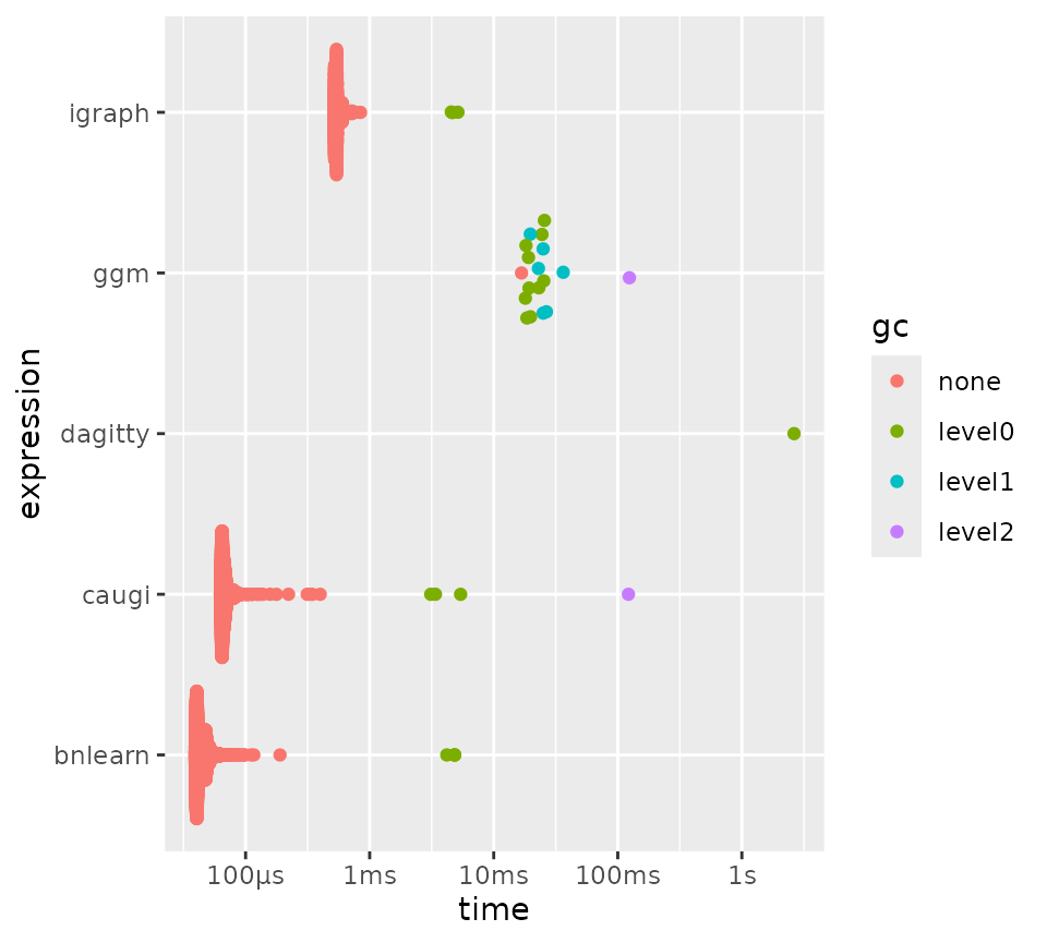

Benchmarking parents/children queries for different packages.

As you can see, caugi followed by bnlearn performs the best for this particular example. In our next experiment, however, we will examine if this extends to different graph sizes and densities, by parameterizing our benchmark over n and p. Note that we adjust p as a function of n to keep the graphs reasonably sparse.

bm_parents_children_np <-
  bench::press(
    n = c(10, 100, 500, 1000, 5000, 10000),
    p = c(0.5, 0.9),
    {
      p_mod <- 10 * log10(n) / n * p
      graphs <- generate_graphs(n, p = p_mod)
      cg <- graphs$cg
      ig <- graphs$ig
      ggmg <- graphs$ggmg
      bng <- graphs$bng
      dg <- graphs$dg

      test_node_index <- sample(n, 1)
      test_node_name <- paste0("V", test_node_index)

      bench::mark(
        caugi = {
          caugi::parents(cg, test_node_name)
          caugi::children(cg, test_node_name)
        },
        igraph = {
          igraph::neighbors(ig, test_node_name, mode = "in")
          igraph::neighbors(ig, test_node_name, mode = "out")
        },
        bnlearn = {
          bnlearn::parents(bng, test_node_name)
          bnlearn::children(bng, test_node_name)
        },
        ggm = {
          ggm::pa(test_node_name, ggmg)
          ggm::ch(test_node_name, ggmg)
        },
        dagitty = {
          dagitty::parents(dg, test_node_name)
          dagitty::children(dg, test_node_name)
        },
        check = FALSE # igraph returns igraph object
      )
    },
    .quiet = TRUE
  )

Next, we plot the benchmark results. As you can see, bnlearn performs worse as graph size and density increases, whereas caugi is almost unaffected by these parameters, outperforming all other packages when graphs get larger and denser. dagitty and ggm perform worst overall, quickly becoming infeasible for larger graphs.

Parameterized benchmarking of parents/children queries.

For ancestors and descendants, we see that caugi outperforms all other packages by a several magnitudes, except for igraph, which it still beats, but by a smaller margin:

bm_ancestors_descendants <- bench::mark(
  caugi = {
    caugi::ancestors(cg, "V500")
    caugi::descendants(cg, "V500")
  },
  igraph = {
    igraph::subcomponent(ig, "V500", mode = "in")
    igraph::subcomponent(ig, "V500", mode = "out")
  },
  bnlearn = {
    bnlearn::ancestors(bng, "V500")
    bnlearn::descendants(bng, "V500")
  },
  dagitty = {
    dagitty::ancestors(dg, "V500")
    dagitty::descendants(dg, "V500")
  },
  check = FALSE # dagitty returns V500 as well and igraph returns an igraph
)

plot(bm_ancestors_descendants)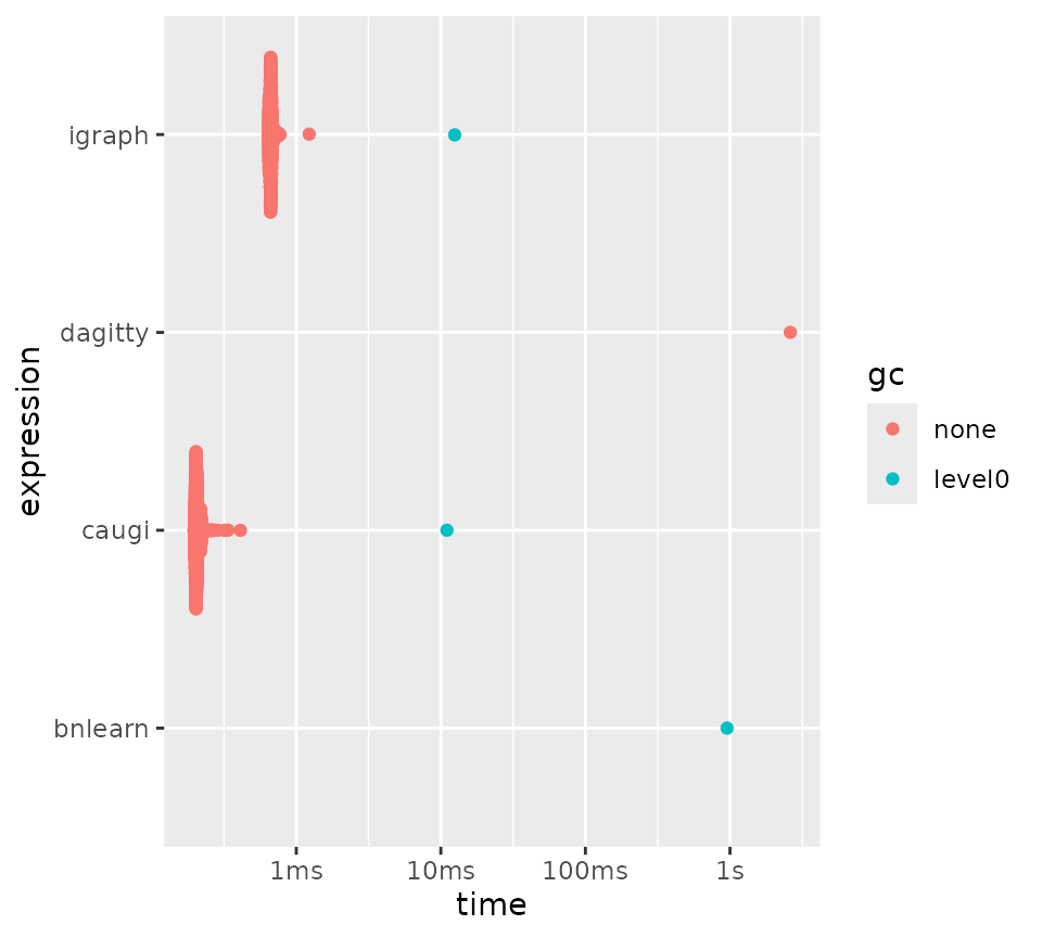

Benchmarking ancestors/descendants queries for different packages.

D-separation

Using the graph from before, we obtain a valid adjustment set and then check for d-separation.

valid_adjustment_set <- caugi::adjustment_set(
  cg,
  "V500",
  "V681",
  type = "backdoor"
)
valid_adjustment_set
#>   [1] "V7"    "V15"   "V18"   "V24"   "V33"   "V34"   "V68"   "V88"   "V93"  
#>  [10] "V121"  "V134"  "V157"  "V168"  "V197"  "V202"  "V206"  "V213"  "V232" 
#>  [19] "V262"  "V287"  "V290"  "V291"  "V302"  "V306"  "V314"  "V330"  "V332" 
#>  [28] "V342"  "V361"  "V363"  "V368"  "V369"  "V371"  "V385"  "V389"  "V393" 
#>  [37] "V409"  "V416"  "V422"  "V425"  "V429"  "V437"  "V444"  "V457"  "V469" 
#>  [46] "V476"  "V480"  "V493"  "V504"  "V510"  "V514"  "V522"  "V530"  "V543" 
#>  [55] "V555"  "V557"  "V560"  "V564"  "V570"  "V581"  "V588"  "V596"  "V607" 
#>  [64] "V620"  "V621"  "V636"  "V641"  "V652"  "V653"  "V660"  "V664"  "V669" 
#>  [73] "V673"  "V677"  "V697"  "V701"  "V707"  "V735"  "V743"  "V748"  "V768" 
#>  [82] "V785"  "V835"  "V836"  "V844"  "V847"  "V890"  "V893"  "V900"  "V911" 
#>  [91] "V912"  "V923"  "V924"  "V927"  "V943"  "V950"  "V964"  "V966"  "V973" 
#> [100] "V974"  "V989"  "V991"  "V996"  "V1000"

bm_dsep <- bench::mark(
  caugi = caugi::d_separated(cg, "V500", "V681", valid_adjustment_set),
  bnlearn = bnlearn::dsep(bng, "V500", "V681", valid_adjustment_set),
  dagitty = dagitty::dseparated(dg, "V500", "V681", valid_adjustment_set)
)

plot(bm_dsep)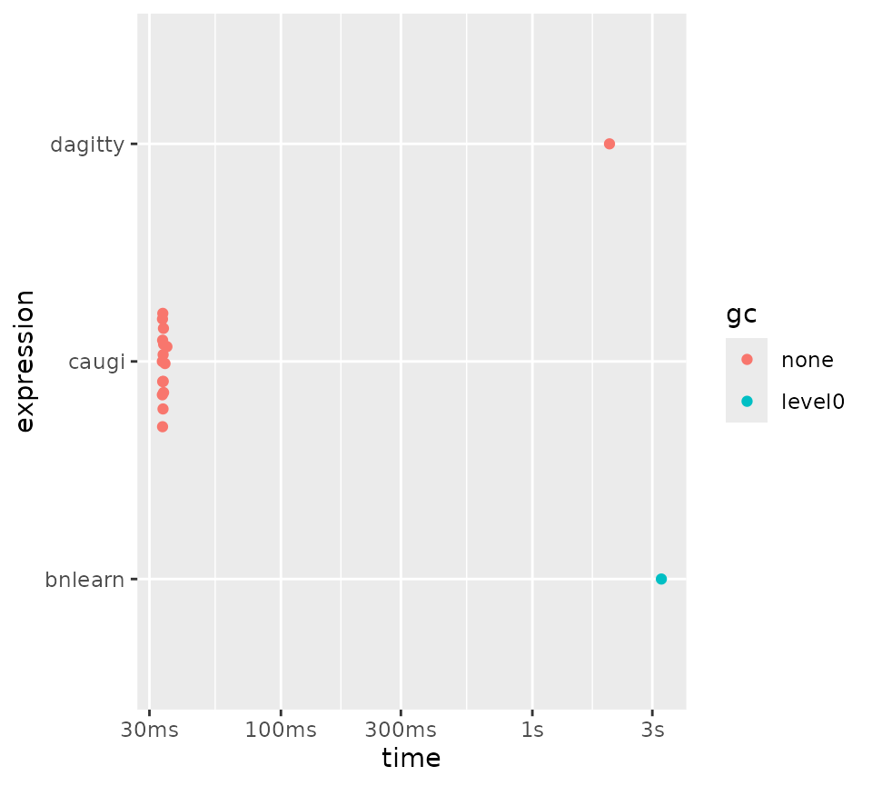

Benchmarks for obtaining a valid adjustment set for d-separation.

We see that caugi again outperforms the other packages by a large margin.

Subgraph (building)

Subgraph extraction is where we explicitly test graph building performance. When extracting a subgraph, caugi must construct a new graph object with its CSR indexes, so this benchmark captures the cost of that frontloaded work. Note that caugi::subgraph() is called on a graph that has already been built.

subgraph_nodes_index <- sample.int(1000, 500)
subgraph_nodes <- paste0("V", subgraph_nodes_index)

bm_subgraph <- bench::mark(
  caugi = {
    sg <- caugi::subgraph(cg, subgraph_nodes)
    caugi::build(sg)
  },
  igraph = {
    igraph::subgraph(ig, subgraph_nodes)
  },
  bnlearn = {
    bnlearn::subgraph(bng, subgraph_nodes)
  },
  check = FALSE
)

plot(bm_subgraph)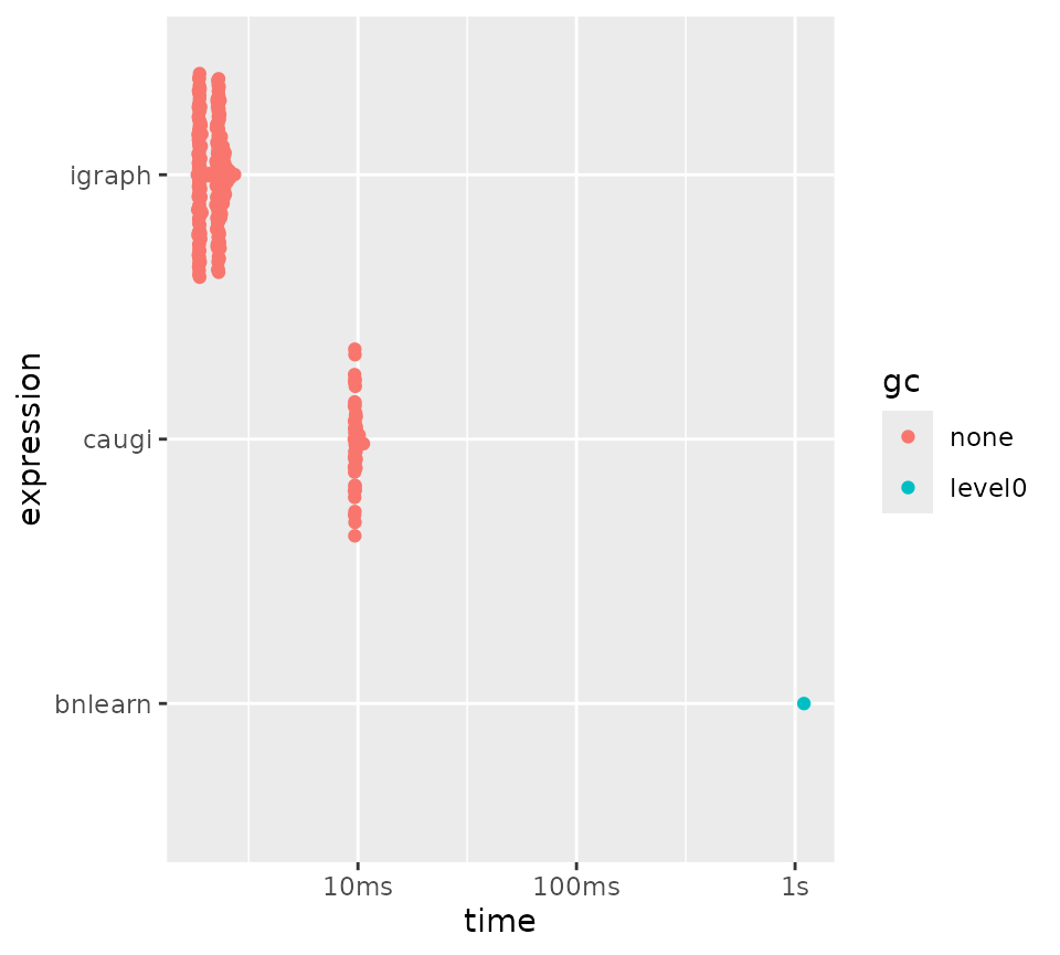

Benchmarking subgraph extraction for different packages.

To make the comparison more demanding, we also benchmark two larger settings where we only compare caugi and igraph directly. This isolates subgraph building performance at scale without the conversion overhead of other packages.

n_large <- 10000
sub_frac <- 0.10
sub_k <- as.integer(n_large * sub_frac)

cg_large_sparse <- caugi::generate_graph(n = n_large, p = 0.05, class = "DAG")
caugi::build(cg_large_sparse)
ig_large_sparse <- caugi::as_igraph(cg_large_sparse)
sub_idx_sparse <- sample.int(n_large, sub_k)
sub_nodes_sparse <- paste0("V", sub_idx_sparse)

bm_subgraph_large_sparse <- bench::mark(
  caugi = {
    sg <- caugi::subgraph(cg_large_sparse, sub_nodes_sparse)
    caugi::build(sg)
  },
  igraph = {
    igraph::subgraph(ig_large_sparse, sub_nodes_sparse)
  },
  check = FALSE,
  iterations = 30
)

plot(bm_subgraph_large_sparse)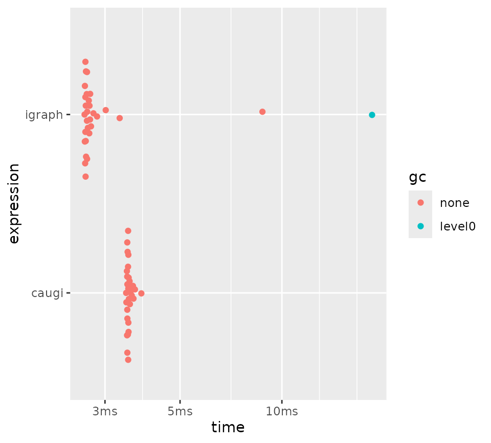

Subgraph extraction on a large sparse graph (n = 10000, p = 0.05).

cg_large_dense <- caugi::generate_graph(n = n_large, p = 0.25, class = "DAG")
caugi::build(cg_large_dense)
ig_large_dense <- caugi::as_igraph(cg_large_dense)
sub_idx_dense <- sample.int(n_large, sub_k)
sub_nodes_dense <- paste0("V", sub_idx_dense)

bm_subgraph_large_dense <- bench::mark(
  caugi = {
    sg <- caugi::subgraph(cg_large_dense, sub_nodes_dense)
    caugi::build(sg)
  },
  igraph = {
    igraph::subgraph(ig_large_dense, sub_nodes_dense)
  },
  check = FALSE,
  iterations = 20
)

plot(bm_subgraph_large_dense)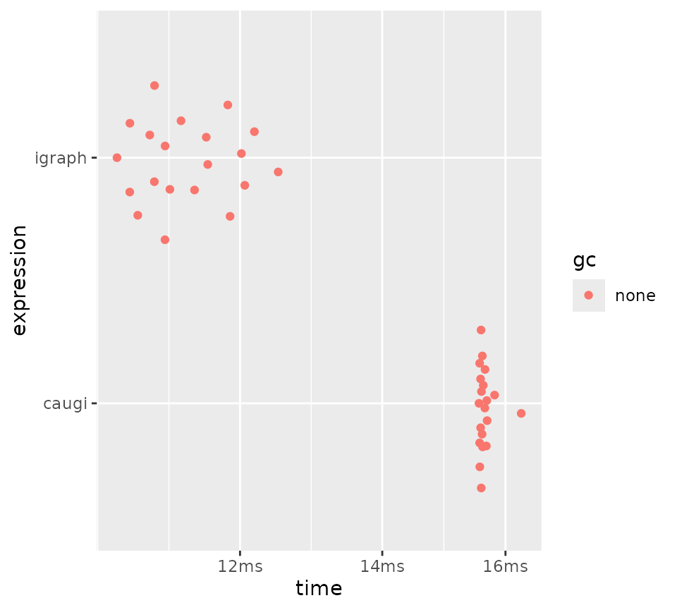

Subgraph extraction on a large dense graph (n = 10000, p = 0.25).

We see that caugi is competitive with igraph for subgraph extraction, even though caugi must rebuild its full CSR representation for the result. igraph does still have a slight edge. ### Session info

sessionInfo()
#> R version 4.6.0 (2026-04-24)
#> Platform: x86_64-pc-linux-gnu
#> Running under: Ubuntu 24.04.4 LTS
#> 
#> Matrix products: default
#> BLAS:   /usr/lib/x86_64-linux-gnu/openblas-pthread/libblas.so.3 
#> LAPACK: /usr/lib/x86_64-linux-gnu/openblas-pthread/libopenblasp-r0.3.26.so;  LAPACK version 3.12.0
#> 
#> locale:
#>  [1] LC_CTYPE=C.UTF-8       LC_NUMERIC=C           LC_TIME=C.UTF-8       
#>  [4] LC_COLLATE=C.UTF-8     LC_MONETARY=C.UTF-8    LC_MESSAGES=C.UTF-8   
#>  [7] LC_PAPER=C.UTF-8       LC_NAME=C              LC_ADDRESS=C          
#> [10] LC_TELEPHONE=C         LC_MEASUREMENT=C.UTF-8 LC_IDENTIFICATION=C   
#> 
#> time zone: UTC
#> tzcode source: system (glibc)
#> 
#> attached base packages:
#> [1] stats     graphics  grDevices utils     datasets  methods   base     
#> 
#> other attached packages:
#> [1] ggplot2_4.0.3
#> 
#> loaded via a namespace (and not attached):
#>  [1] tidyr_1.3.2         sass_0.4.10         generics_0.1.4     
#>  [4] digest_0.6.39       magrittr_2.0.5      evaluate_1.0.5     
#>  [7] grid_4.6.0          RColorBrewer_1.1-3  fastmap_1.2.0      
#> [10] jsonlite_2.0.0      graph_1.90.0        bench_1.1.4        
#> [13] BiocManager_1.30.27 purrr_1.2.2         dagitty_0.3-4      
#> [16] scales_1.4.0        textshaping_1.0.5   jquerylib_0.1.4    
#> [19] cli_3.6.6           rlang_1.2.0         ggm_2.5.2          
#> [22] bnlearn_5.1         withr_3.0.2         cachem_1.1.0       
#> [25] yaml_2.3.12         otel_0.2.0          ggbeeswarm_0.7.3   
#> [28] tools_4.6.0         parallel_4.6.0      dplyr_1.2.1        
#> [31] profmem_0.7.0       boot_1.3-32         BiocGenerics_0.58.0
#> [34] curl_7.1.0          vctrs_0.7.3         R6_2.6.1           
#> [37] stats4_4.6.0        lifecycle_1.0.5     fs_2.1.0           
#> [40] V8_8.2.0            htmlwidgets_1.6.4   vipor_0.4.7        
#> [43] MASS_7.3-65         ragg_1.5.2          beeswarm_0.4.0     
#> [46] pkgconfig_2.0.3     desc_1.4.3          pkgdown_2.2.0      
#> [49] pillar_1.11.1       bslib_0.10.0        gtable_0.3.6       
#> [52] data.table_1.18.2.1 glue_1.8.1          Rcpp_1.1.1-1.1     
#> [55] systemfonts_1.3.2   tidyselect_1.2.1    xfun_0.57          
#> [58] tibble_3.3.1        knitr_1.51          farver_2.1.2       
#> [61] htmltools_0.5.9     igraph_2.3.1        labeling_0.4.3     
#> [64] rmarkdown_2.31      caugi_1.2.0         compiler_4.6.0     
#> [67] S7_0.2.2